Predicting the Orbital Obliquities of Exoplanets Using Machine Learning

In this project, I applied machine learning to explore an interesting question in astronomy: Can we predict the orbital obliquities of exoplanets using their host stars' properties and planetary system features? Orbital obliquity—the angle between a planet's orbital plane and the equator of its host star—offers crucial insights into planetary formation and evolution. Here's how I approached this challenge using a random forest regression model.
Data Collection and Pre-processing
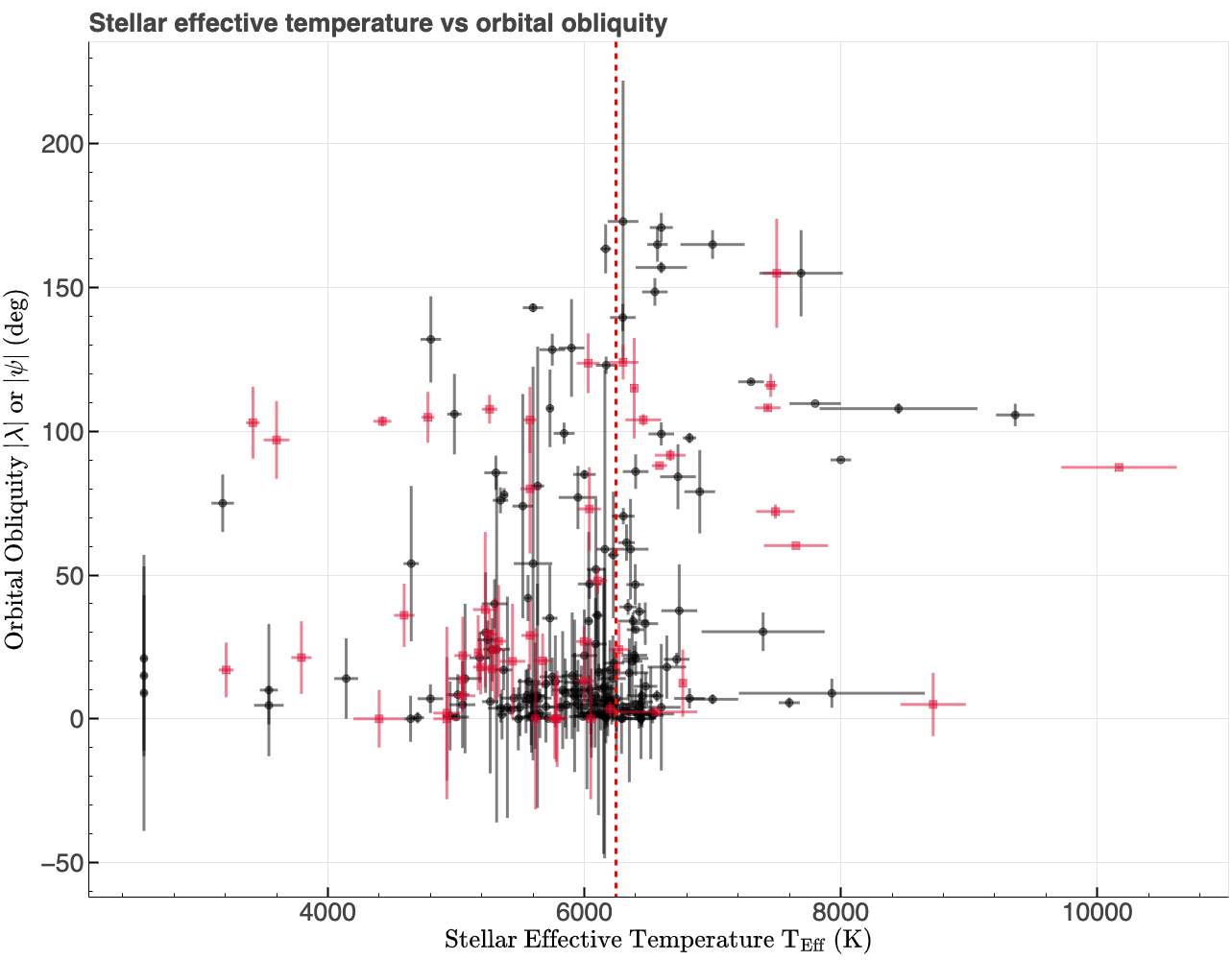
The first step involved obtaining data from two databases: the catalog of the physical properties of transiting planetary systems (TEPCat) and the NASA Exoplanet Archive. These sources provided the required properties of the exoplanets and their host star's to build a machine learning model, including, for example, the masses, radii, orbital distances, and orbital obliquities. However, the sample size of planets with measured orbital obliquities was small and the measurements came with significant uncertainties. Additionally, the dataset is somewhat imbalanced, there are more than double the number of planets on low obliquity orbits compared to high obliquity orbits as shown in the figure below.

To address these challenges, I employed a novel approach: simulation and sampling within error bars (1 σ uncertainties). By using the reported uncertainties for key features, I generated additional synthetic data points. This not only expanded the dataset but also introduced additional variability to hopefully allow the model to capture the underlying patterns more effectively. However, this approach does not solve the issue with data imbalance, but still could be particularly valuable when dealing with sparse datasets.
The code for obtaining the datasets, cleaning the datasets, and building the machine learning models is available as Jupyter notebooks on GitHub, which can be found here for the random forest regression model and here for the random forest classification model (see parts 4 and 5 of this blog post series when they become available). To obtain the dataset from the NASA Exoplanet Archive, I used the Table Access Protocol (TAP) service with SQL commands (see Predicting the Orbital Obliquities of Exoplanets Using Machine Learning Part 2 In-depth for more details). The dataset from TEPCat was obtained using a simple HTTP GET request:
requests.get("https://www.astro.keele.ac.uk/jkt/tepcat/obliquity.csv")
Building the Random Forest Model
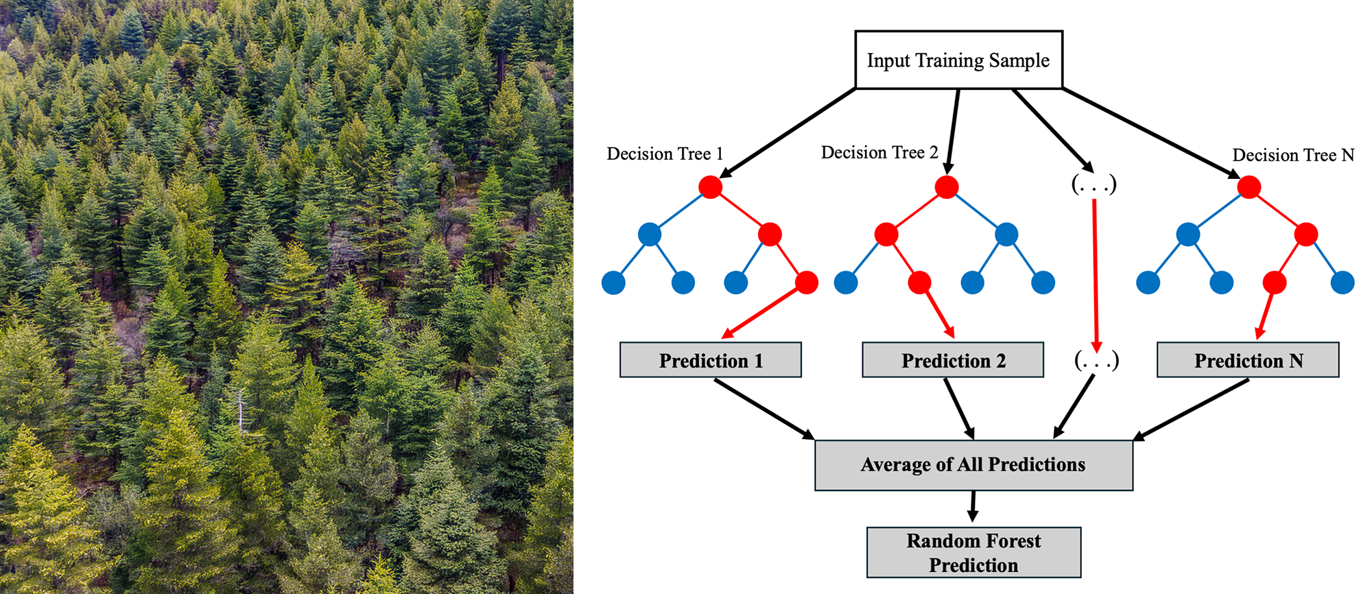
Using Python and the Scikit-learn library, I constructed a random forest regression model. Random forests are ensemble models that aggregate predictions from multiple decision trees to improve accuracy and reduce overfitting (see illustrative figure at the top of the page).
The model was trained on a set of 16 features, including:
- Planetary properties such as mass, radius, orbital period, and eccentricity.
- Stellar properties like mass, radius, temperature, age, and metallicity.
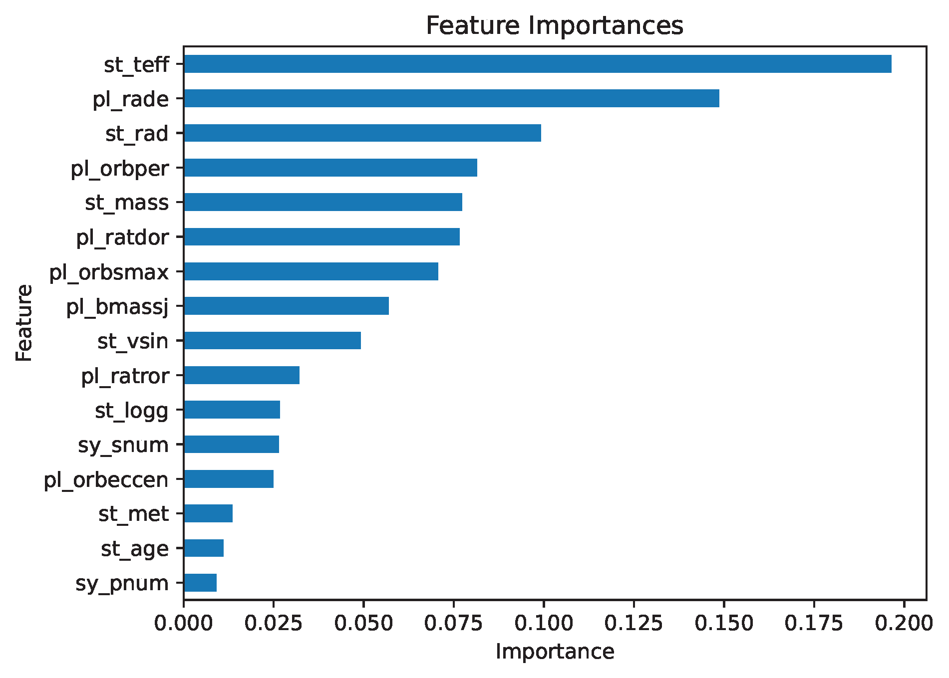
Despite my best efforts, the model faced limitations due to the inherent sparsity and noise in the data. While it could identify some broad trends, the predictions for individual orbital obliquities lacked the precision necessary for application to new data or drawing robust scientific conclusions. However, the process did highlight some of the features most likely to influence orbital obliquity. For example, stellar effective temperature emerged as the most significant predictor (see feature importance plot below), offering valuable insights and potential directions for this project.

Key Results and Insights
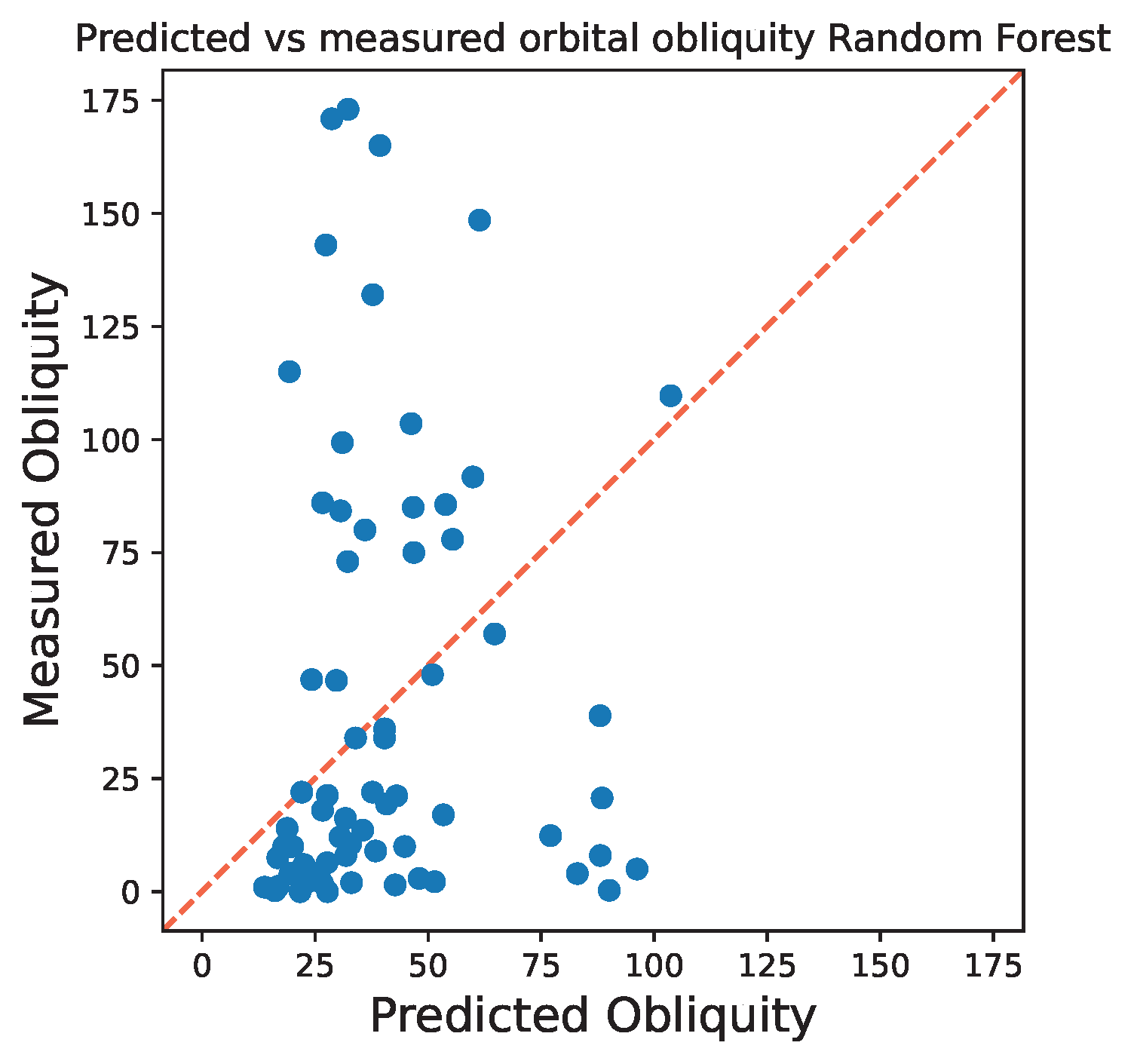
Unfortunately, the random forest regression model performed poorly in predicting obliquities, with an R2 (R squared) score of 0.26. Generally, a R2 score above 0.8 is a good indication that the model is performing well in making accurate predictions. Two likely reasons for this are: (1) the dataset is imbalanced, with about two-thirds of planets on low-obliquity orbits, and (2) the features used are weak predictors of obliquity. Both factors likely contribute to the model's limited performance. To visually assess my model's performance, I plotted the predicted vs. measured obliquities that includes a diagonal reference line where predicted = measured (error bar version here). If the predicted obliquities from the model matches the actual (true) values, then the points on the figure would fall along the diagonal, indicating accurate predictions. However, as shown in the figure, the model significantly underpredicts high obliquities and overpredicts low obliquities.

Although the model's predictive power was limited, the project provided several valuable insights:
- The importance of robust and comprehensive datasets: The model's performance highlights the need for a larger, more complete dataset with smaller uncertainties. This challenge is common in astronomy, where data can be sparse and have large uncertainties, and is equally critical in data science applications.
- Addressing dataset imbalances: Imbalanced datasets can bias machine learning models, making it difficult to achieve accurate predictions across a broad range of outcomes. Ensuring balanced representation within the dataset is crucial for reliable model performance.
- Feature selection and relevance: Including features that strongly correlate with the target variable—in this case, orbital obliquity—is fundamental for building an accurate and robust model. Irrelevant or weakly related features can dilute the predictive power of the model.
- Deep understanding of data: A thorough understanding of the dataset, including the physical relationships and correlations among features, is essential before applying machine learning techniques. This step ensures that the model is grounded in the physics and context of the problem, rather than purely statistical patterns.
Summary and Next Steps
This project demonstrates the potential and pitfalls of applying machine learning techniques to problems in astronomy and data science. While data-driven approaches offer the potential to uncover new insights, their success depends heavily on integration with domain-specific knowledge (thorough understanding of the data and the problem), especially when working with sparse or noisy datasets. Future efforts could focus on expanding the sample of data (in particular when new data sources become available), optimizing feature selection and/or engineering new features to better capture relevant patterns, or implementing other advanced machine learning models better suited to this problem to enhance predictive accuracy.
In Part 3 of this blog series, I will share the steps I've taken to refine the random forest regression model and improve its performance! If you'd like to delve deeper into the methodology, code, or results, you can read the full article on my website: Predicting the Orbital Obliquities of Exoplanets Using Machine Learning Part 2 In-depth.
Summary of the skills applied in this work: Python programming, Table Access Protocol (TAP), Application Programming Interface (API), Structured Query Language (SQL), Data Exploration, Data Visualization, Handling Missing Values (Data Imputation), Data Augmentation, Machine Learning, Random Forest Regression, K-Fold Cross-Validation.
< Previous Post | Data Science Home Page ⌂ | Next Post >