Predicting the Orbital Obliquities of Exoplanets Using Machine Learning

Illustration of a random forest model consisting of N number of decision trees, with each tree consisting of M number of branches (or nodes), similar to how a forest consists of many trees and each tree consists of many branches. The nodes within each decision tree are used to make a prediction, and all of the predictions are averaged together to produce a final result. The red path taken in each decision tree is where specific criteria are met that result in a prediction. Image credit: Brett Addison.

 

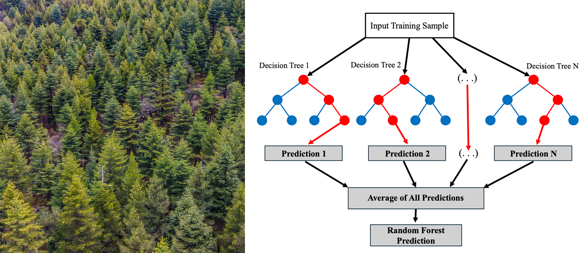
In this project, I have constructed random forest regression and classification models using the Python library Scikit-learn to try to predict orbital obliquity. Part 2 of this blog post series is about obtaining the datasets I will be using to build the predictive models on, cleaning the datasets, and then my first attempt to build a random forest regression model to predict the orbital obliquities of exoplanets.

 

What is Random Forest Regression?

For readers unfamiliar with machine learning and its applications in data science, you might wonder: what is random forest regression, and why use it to predict the orbital obliquities of exoplanets? Great questions!

 

Machine learning (ML) is a subfield of artificial intelligence (AI) focused on enabling computers to learn and perform tasks without being given explicit instructions (see short overview article on ML given by Sara Brown). This is accomplished using various algorithms and statistical models that analyze data, uncover patterns, and make predictions on new, unseen data. Random forest is one such versatile and widely used ML algorithm in the data science community (e.g., see articles given by AnalytixLabs and IBM), making it an excellent choice for this project.

 

At its core, random forest is an ensemble learning method based on decision trees. A decision tree is a branch-like structure consisting of many nodes (decision points) that split data based on answers to specific questions about features (for this project, exoplanet/host star properties). For example, a node might ask: "Is the host star’s effective temperature greater than 6250K?" Depending on the answer, the algorithm moves to the next node, eventually reaching a leaf (terminal) node where a prediction is made (e.g., in my case, the orbital obliquity angle).

 

Random forest enhances decision trees by using an ensemble of multiple trees (see illustration above), each trained on a randomly selected subset of data (a technique known as bagging). It also introduces feature randomness by selecting a random subset of features to use for each tree. These techniques ensure diversity among the trees, resulting in more robust and accurate predictions. The final prediction is typically the average (for regression) or majority vote (for classification) of all trees in the forest.

 

For the first part of this project, I’m using the regression version of random forest to analyze the relationship between exoplanet and host star properties and quantitatively predict orbital obliquity angles. Later, I’ll apply the classification version to categorize planetary orbits as being aligned or misaligned/highly misaligned. For more detailed overviews on the random forest algorithm, check out excellent tutorials from IBM or YouTube videos by experts like Martin Keen.

 

By leveraging the power of random forest, I aim to uncover meaningful patterns in exoplanetary systems and improve our understanding of their orbital dynamics.

 

Building the Random Forest Model using an Exoplanet Dataset

The obliquity data comes from the catalog of the physical properties of transiting planetary systems (TEPCat), and most of the other planetary and host star properties come from the NASA Exoplanet Archive. The code for obtaining the dataset, cleaning the dataset, and building the machine learning models is available as Jupyter notebooks on GitHub, which can be found here for the random forest regression model and here for the random forest classification model (see parts 4 and 5 of this blog post series when they become available).

 

Step 1: Obtaining Datasets

The first step in this project is obtaining the datasets required to train the models. As mentioned earlier, the obliquity dataset comes from TEPCat, and the exoplanet/host star properties dataset comes from the NASA Exoplanet Archive. TEPCat provides the obliquity dataset in both HTML and text formats, which can be downloaded using a simple HTTP GET request:

requests.get("https://www.astro.keele.ac.uk/jkt/tepcat/obliquity.csv")

 

Once downloaded, the obliquity dataset is stored in a Pandas DataFrame for easy cleaning and model fitting.

 

For the exoplanet/host star properties dataset, I used the Table Access Protocol (TAP) service, a convenient and preferred method recommended by the NASA Exoplanet Archive. While an API is also available, it is being phased out in favor of TAP, and the specific table needed for this project is accessible only via TAP (an example API call is also included in the Jupyter notebook for reference). To use TAP in Python, I used the PyVO package to construct and execute a query. This query utilized SQL commands like SELECT (to specify the desired columns), FROM (to indicate the table), and WHERE (to filter rows based on specific conditions). The resulting dataset was stored in a Pandas DataFrame. Below is an example query:

 

 

The selected columns include those likely to serve as features in the machine learning model. Columns unrelated to predicting obliquity were omitted to streamline the dataset. Additionally, specific filtering conditions were applied:

• default_flag = 1: Ensures the use of default (preferred) values.
• tran_flag = 1: Includes only transiting planets (orbital obliquities are measured only for transiting exoplanets).
• pl_controv_flag = 0: Excludes controversial planets.

 

Step 2: Cleaning Datasets & Merging Tables

After obtaining the two tables, obliquity and exoplanet/host star properties, we need to clean the datasets and then merge the two tables into one. This merged table will allow us to train our machine learning models and predict the orbital obliquities of exoplanets.

1. The first step is to remove unwanted rows in the obliquity table. Many planets have multiple entries because the TEPCat obliquity table contains nearly all published measurements. We only want the preferred or accepted values, which are typically the most recent measurements but not always. Thankfully, TEPCat includes a Pflag column indicating whether a row contains the preferred value (Pflag = y). Using this filter reduces the number of rows from 387 to 238. Note that this step has already been done for the exoplanet/host star properties table by specifying the condition default_flag = 1 in the SQL TAP query.

 



The first five rows and all of the columns in the obliquity table from TEPCat. Note the format of the planet names under the column ‘System’ and the ‘Pflag’ column, which indicates which rows contain the preferred values. Image credit: Brett Addison.

 

2. Next, we fix the planet names in the obliquity table to match the format in the exoplanet/host star properties table to allow crossmatching. The obliquity table uses underscores ('_') instead of spaces and doesn’t always include planet letters ('b', 'c', etc.). A function called format_planet_name was created to standardize the names. However, crossmatching still fails for some planets due to naming inconsistencies between astronomical databases. A workaround involves querying the SIMBAD database for alternate names using the Python package Astroquery. The function query_simbad_for_names loops through unmatched planet names, queries SIMBAD (via Simbad.query_objectids), and retrieves possible name matches. This method successfully crossmatched 8 out of 17 previously unmatched planets, resulting in 226 matched planets overall.

 

3. With standardized names, the two tables are merged into a single dataframe using the Pandas merge function. After merging, further cleaning is required to handle overlapping columns, such as Teff, errup, and errdn (from the obliquity table) versus st_teff, st_tefferr1, and st_tefferr2 (from the exoplanet/host star properties table). Preference is given to values from the exoplanet/host star properties table since the NASA Exoplanet Archive has the most up-to-date values for the stellar effective temperature. When lower (errdn) and upper (errup) uncertainties are provided, their average is taken to simplify the analyses later on. If a parameter lacks uncertainty values, it is assumed that the given value represents a 1σ upper limit. In such cases, the uncertainty is set equal to the parameter value. The uncertainties on the parameters will be used to augment (generate) simulated data. This is done to incorporate the uncertainties of the target and features into the random forest model and increase the sample size, given the small sample (226) of planets in the dataset.

 

4. Next, the obliquity values (λ and ψ) are adjusted to fall within the range of 0° to 180°, as only values within this range are physically meaningful. Adjustments include:

   • Negative values between 0° and -180° are converted to their absolute values (e.g., -80° becomes 80°).
   • Values between -180° and -360° are adjusted by adding 360° (e.g., -270° becomes 90°).
   • Values greater than 180° are adjusted by subtracting them from 360° (e.g., 270° becomes 90°).

 

5. Finally, unnecessary columns are dropped. Columns such as Pflag, default_flag, and reference/author fields are removed, as they do not contribute to predictive modeling. Columns with excessive missing values or low predictive power are also excluded. After cleaning, the dataset includes 16 features. Additional features created through feature engineering will be discussed later.

 

	Column Name	Definition	Target or Feature	Numerical or Categorical	Source
1	lambda	Sky-projected obliquity	Target	Numerical	TEPCat
2	psi	True obliquity	Target	Numerical	TEPCat
3	sy_snum	Number of stars in system	Feature	Numerical	NASA
4	sy_pnum	Number of planets in system	Feature	Numerical	NASA
5	pl_orbper	Planet orbital period (days)	Feature	Numerical	NASA
6	pl_orbsmax	Planet semi-major axis (AU)	Feature	Numerical	NASA
7	pl_rade	Planet radius (Earth radii)	Feature	Numerical	NASA
8	pl_bmassj	Planet mass (Jupiter masses)	Feature	Numerical	NASA
9	pl_orbeccen	Planet orbital eccentricity	Feature	Numerical	NASA
10	pl_ratdor	Ratio of planet semi-major axis to stellar radius	Feature	Numerical	NASA
11	pl_ratror	Ratio of planet to stellar radius	Feature	Numerical	NASA
12	st_teff	Stellar effective temperature	Feature	Numerical	NASA/TEPCat
13	st_rad	Stellar radius (Solar radii)	Feature	Numerical	NASA
14	st_mass	Stellar mass (Solar masses)	Feature	Numerical	NASA
15	st_met	Stellar metallicity (dex)	Feature	Numerical	NASA
16	st_logg	Stellar surface gravity (log10(cm/s**2))	Feature	Numerical	NASA
17	st_age	Stellar age (Gyr)	Feature	Numerical	NASA
18	st_vsin	Stellar rotational velocity (km/s)	Feature	Numerical	NASA

 

Step 3: Data Exploration, Visualization, and Handling Missing Values

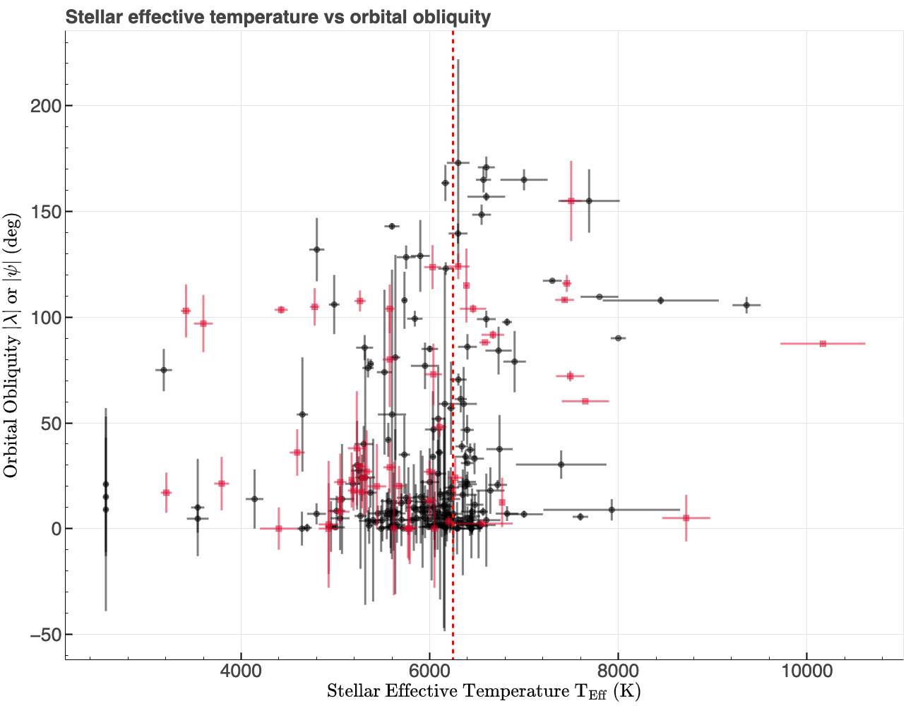
With the dataset mostly cleaned, it’s time to explore it for trends and correlations before training any models. In particular, we will examine the relationships between some of the parameters and orbital obliquity. A notable correlation in the astronomical literature is between stellar effective temperature and orbital obliquity, where hotter stars tend to host more highly misaligned planets (e.g., Winn et al. 2010, Albrecht et al. 2022). Below is a plot of effective temperature versus orbital obliquity. While no strong correlation is evident, closer inspection suggests that stars hotter than the Kraft Break (~6250K, Kraft 1967; ~6550K, Beyer and White 2024) may host a higher fraction of misaligned planets. This boundary (as indicated by the red vertical dashed line in the figure below) separates cooler stars with convective envelopes from hotter stars with radiative envelopes. Cool stars are more efficient at realigning high orbital obliquities through tidal interaction between a planet and its star’s convective envelop compared with hot stars that are inefficient at realigning high obliquity orbits due to lack of tides raised in their radiative envelop. Therefore, the effective temperature of the host star could play an important role in predicting orbital obliquities.

 

The sample of exoplanets with measured orbital obliquities, plotted as host star effective temperature vs orbital obliquity. The black points are the projected orbital obliquities while the red points are the true orbital obliquities. The red dashed line is the approximate location of the Kraft Break between cool and hot stars, with and without a convective envelop, respectively. Click on the image to open a larger interactive version of the plot. Image credit: Brett Addison.

 

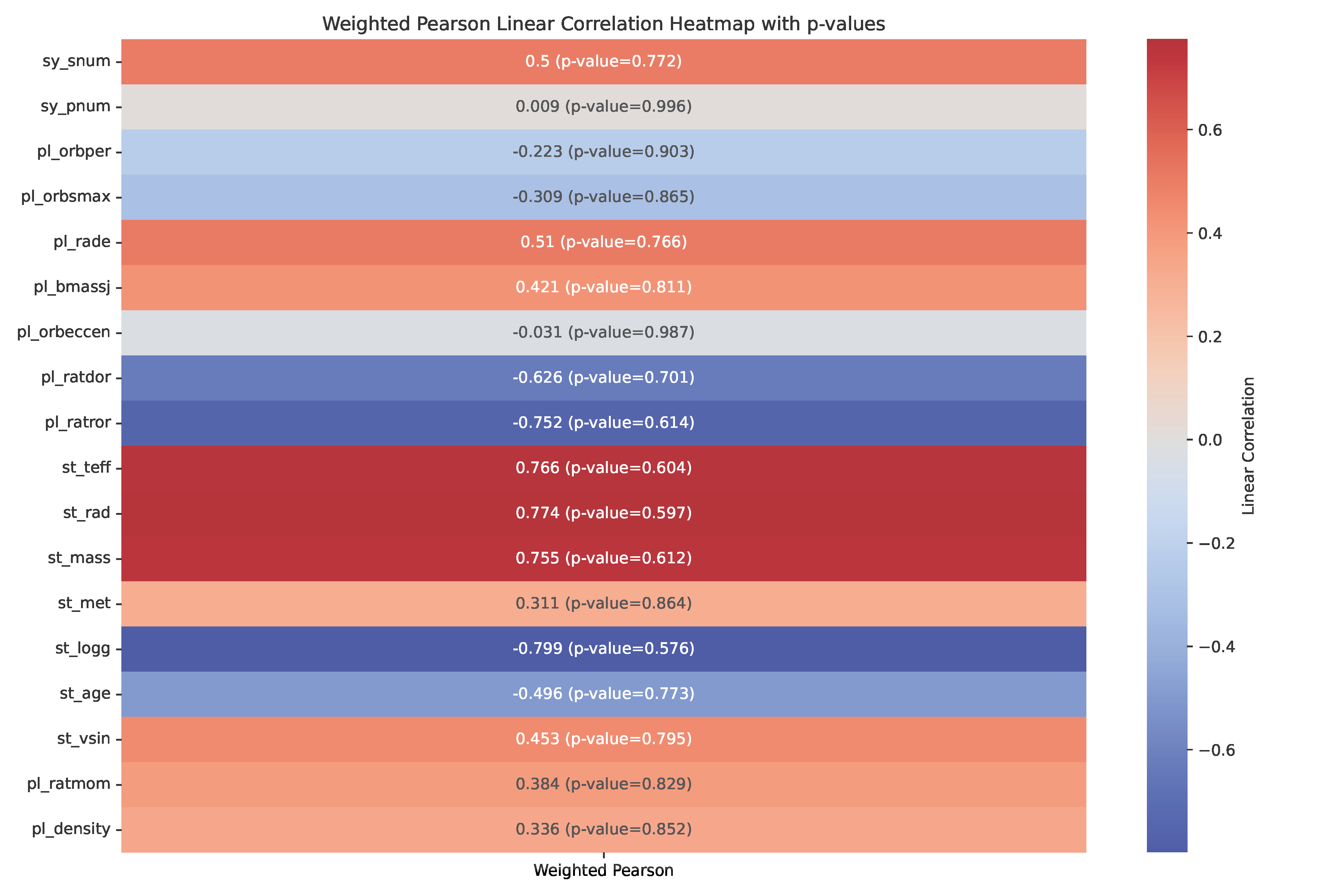
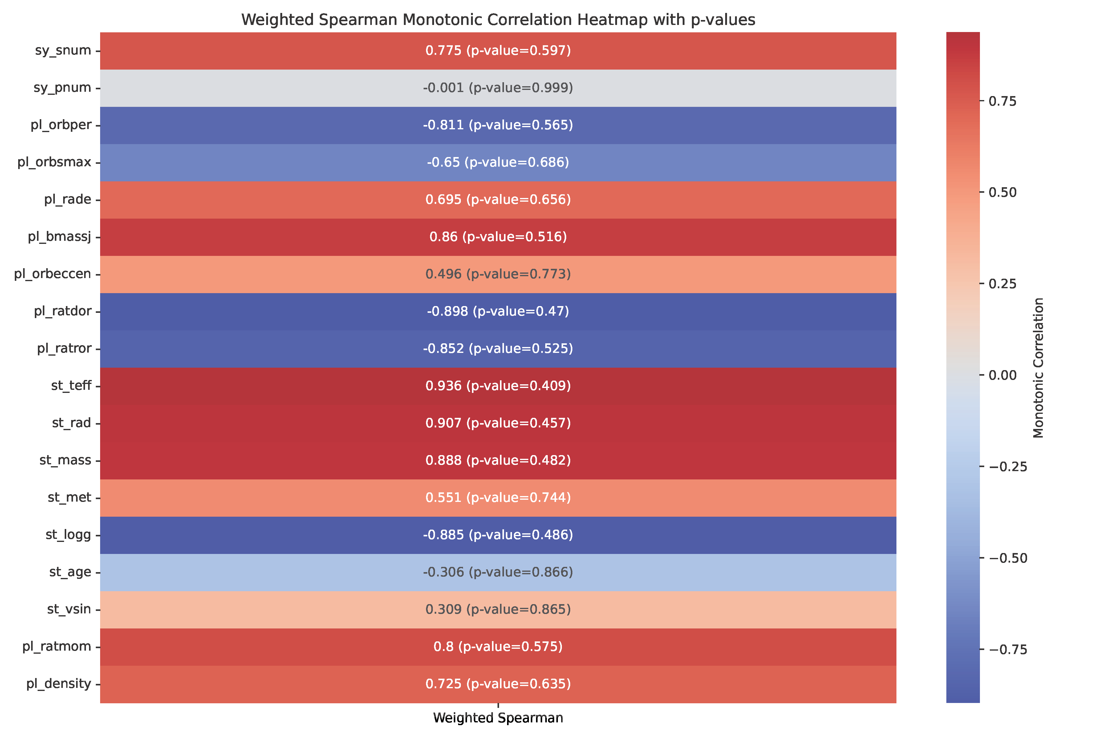
Other parameters, such as system age, planet mass, orbital eccentricity, and orbital distance (or semi-major axis to stellar radius ratio), may also correlate with obliquity. Initial visualizations and correlation heatmaps (Pearson and Spearman) suggest weak relationships, though this will be revisited during modeling. Below I have produced Pearson and Spearman correlation heatmaps as well as calculated the p-values to assess the significance of the correlations.

 

The sample of exoplanets with measured orbital obliquities, plotted as age of the system vs orbital obliquity (left) and planet mass vs orbital obliquity (right). The black points are the projected orbital obliquities while the red points are the true orbital obliquities. Click on the images to open a larger interactive version of the plots. Image credits: Brett Addison.

 

The sample of exoplanets with measured orbital obliquities, plotted as orbital eccentricity vs orbital obliquity (left) and the ratio of the semi-major axis to stellar radius vs orbital obliquity (right). The black points are the projected orbital obliquities while the red points are the true orbital obliquities. Click on the images to open a larger interactive version of the plots. Image credits: Brett Addison.

 

Left: Pearson correlation heatmap showing the strength of the linear correlations between the various parameters and obliquity. P-values were also calculated to assess the significance of the correlations. While the stellar effective temperature has the strongest positive correlation with obliquity at 0.766, its p-value of 0.604 suggest that the correlation is not very significant (note that p-value of 0.05 or lower is considered statistically significant). Right: Spearman correlation heatmap showing the strength of the monotonic (non-linear) correlations between the various parameters and obliquity. P-values were also calculated to assess the significance of the correlations. In this case, the stellar effective temperature has a strong positive correlation with obliquity at 0.936 but its p-value is 0.409, which again suggest that the correlation is not very significant. Click on the images for a larger view of them. Image credits: Brett Addison.

 

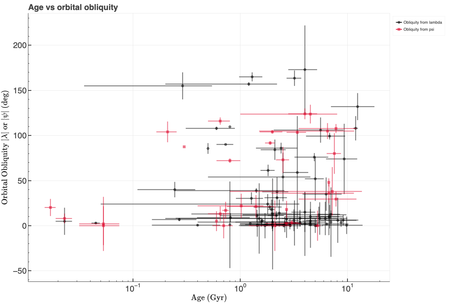
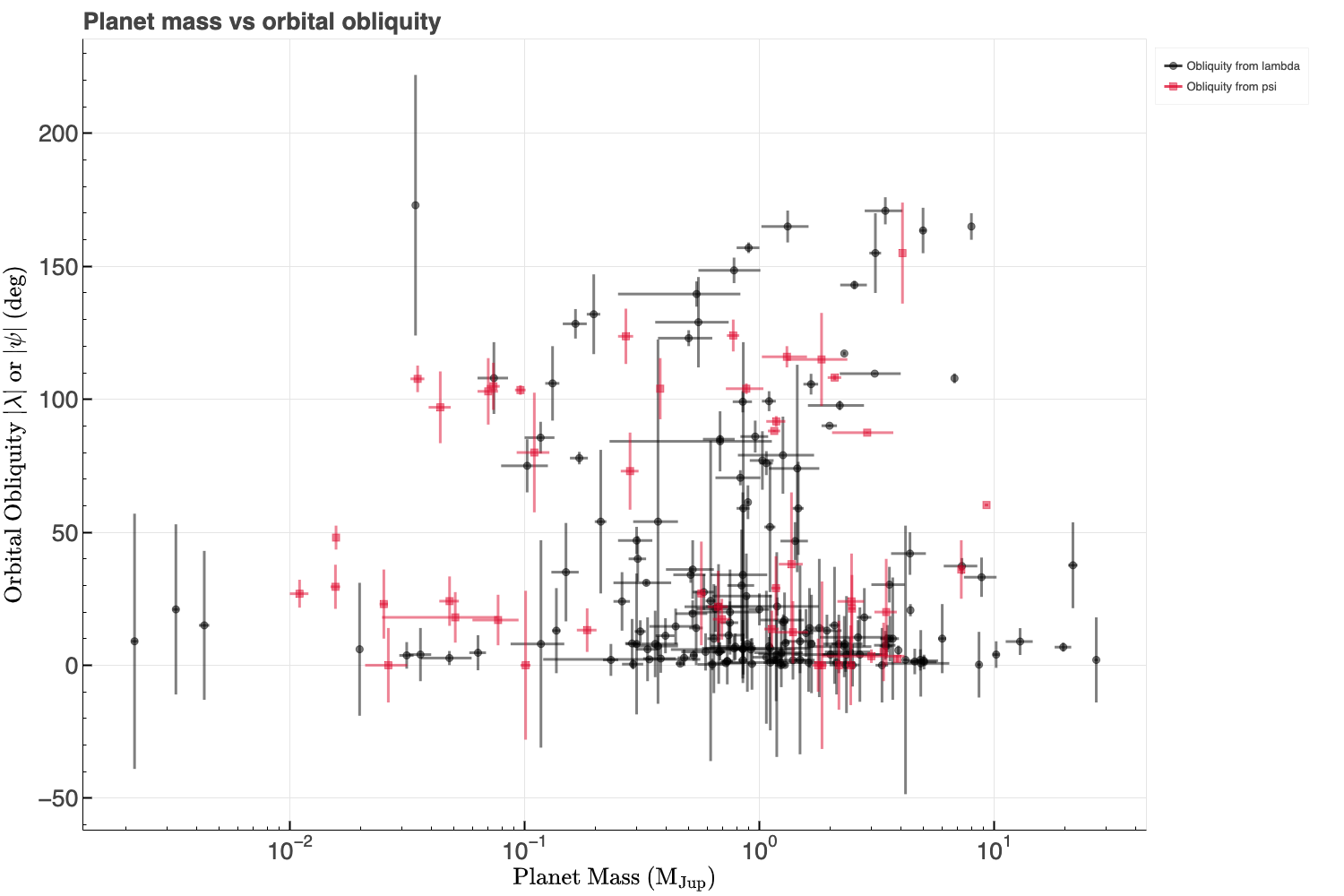
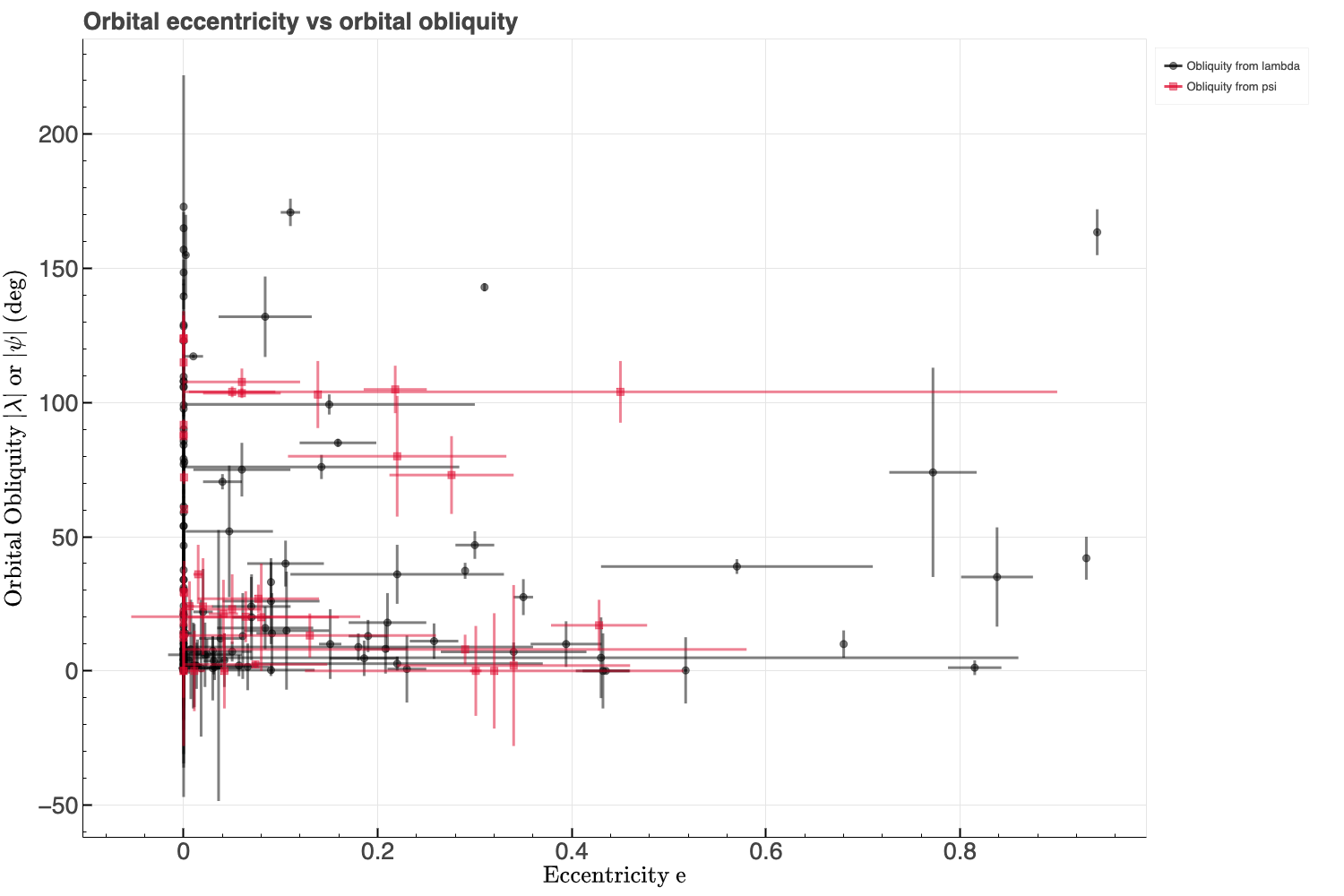
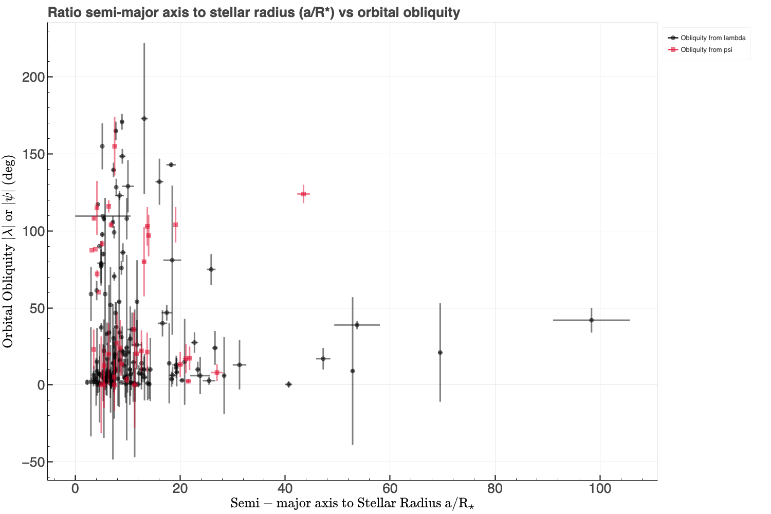
You might have noticed up to this point that obliquity is given as either λ or ψ. Recall that λ is the projected obliquity while ψ is the true obliquity in 3D space. Ideally, we are interested in ψ, but it is often unavailable due to the difficulty of measuring the host star's 3D spin axis orientation. To maximize sample size, I’ve combined λ and ψ into a single target variable (called obliquity), prioritizing ψ when both are available. This approximation is reasonable for the purposes of this project.

 

Before modeling, missing values and categorical data must be dealt with appropriately. In general, ML models such as random forest cannot handle missing values or use categorical features. While the dataset currently lacks categorical features, I’ve included code to handle them using Scikit-learn’s OneHotEncoder. For numerical features with missing values, I impute with the median of the sample—a common approach used in data science as it is robust to outliers and suitable for small sample sizes. While potentially effective as an initial strategy, physical models may offer better imputations, which I will discuss in my next blog post, coming soon.

 

Step 4: Train/Test Dataset Splitting & Data Augmentation

To build and then evaluate the performance of machine learning models, the dataset must be split into training and testing (validation) sets. The training set is used to train the model, while the testing set evaluates how well the model generalizes to unseen data. To start off with, I applied a simple 70/30 train/test split on the obliquity/exoplanet dataset using Scikit-learn’s train_test_split function. I supplied the function with the features, their uncertainties, the target (obliquity), target weights (1/target_uncertainty), and target uncertainties and it returned the training and test sets.

 

Next, I augmented the training dataset to address its small sample size (226 exoplanetary systems) and incorporate parameter uncertainties into the model. Data augmentation involves generating simulated data by sampling distributions centered on feature and target values, with widths defined by 1 σ uncertainties (e.g., see this overview). For this, I created a custom function, augment_data_with_sampling, which generates n simulated rows per training sample. This process expands the dataset, improving the coverage of the parameter space, while accounting for uncertainty, which is particularly important as many features have large uncertainties that should reduce their influence on the model.

 

For this analysis, I generated 100 augmented samples per row, increasing the training set size by a factor of 100. This strikes a balance between improving sample coverage and limiting processing time, as tested against values of 10, 50, 500, and 1000. I should also note that it is crucial to perform data augmentation after splitting the dataset to prevent data leakage, which occurs when augmented samples from the same row appear in both training and testing sets. Such leakage inflates performance metrics by exposing the model to data it has already seen. Furthermore, model validation must be performed on actual, unaugmented (non-simulated) data to ensure reported accuracy reflects real-world performance.

 

One issue to watch out for is unphysical values being generated in the simulated data. For example, planet mass must always be positive and less than the host star’s mass, while eccentricity values must fall between 0 and 1. I implemented constraints in the augmentation function to ensure all simulated data is within physical limits.

 

Step 5: Train & Test Orbital Obliquity Random Forest Regression Model

Now we are at the stage of training and testing a random forest regression model on the exoplanet orbital obliquity dataset. To do this, I have used RandomForestRegressor from Scikit-learn along with the fit and the predict functions. The model was initialized with these key parameters: n_estimators (number of trees), max_features (the maximum number of features to consider for the best split), and random_state (seed for reproducibility). I tested n_estimators values from 100 to 10,000, finding that values above 200 yielded optimal results. For training, I set n_estimators to 1,000, and for cross-validation, I used 200 to balance accuracy and processing time. I set max_features to ‘log2,’ which is effective at balancing model performance and preventing overfitting by limiting the number of features used in splits. Other valid options include integers, fractions, ‘sqrt,’ or None (all features).

 

Once initialized, the model was trained on the dataset using the fit function that included the input features, obliquities (the target), and weights (1/target uncertainty). I then tested the model on the non-augmented testing dataset using the predict function to estimate the obliquities. Performance was evaluated using the following metrics: mean squared error (MSE, the mean squared difference between the predicted and actual values), root mean squared error (RMSE), and R², which measures the proportion of target variance explained by the model features. The R² score was calculated using Scikit-learn’s r2_score by providing it with the observed and predicted obliquities along with the sample weights.

 

Step 6: Results of the Random Forest Regression Model

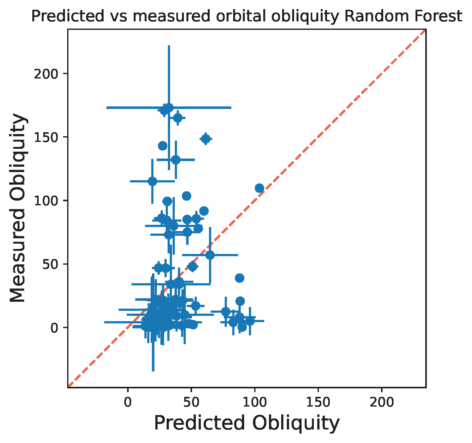
Unfortunately, the random forest regression model performed poorly in predicting obliquities, with an R² score of 0.26. This indicates that less than a quarter of the observed variation in obliquity is explained by the model features. Generally, an R² score above 0.8 is considered good, though R² doesn’t tell the whole story as this metric doesn't fully capture model performance. To assess the model performance further, I plotted the predicted vs. measured obliquities from the test dataset, including a diagonal reference line, as shown below. Ideally, points would align closely with the diagonal, indicating accurate predictions. However, as shown in the figure, the model significantly underpredicts high obliquities and overpredicts low obliquities.

 

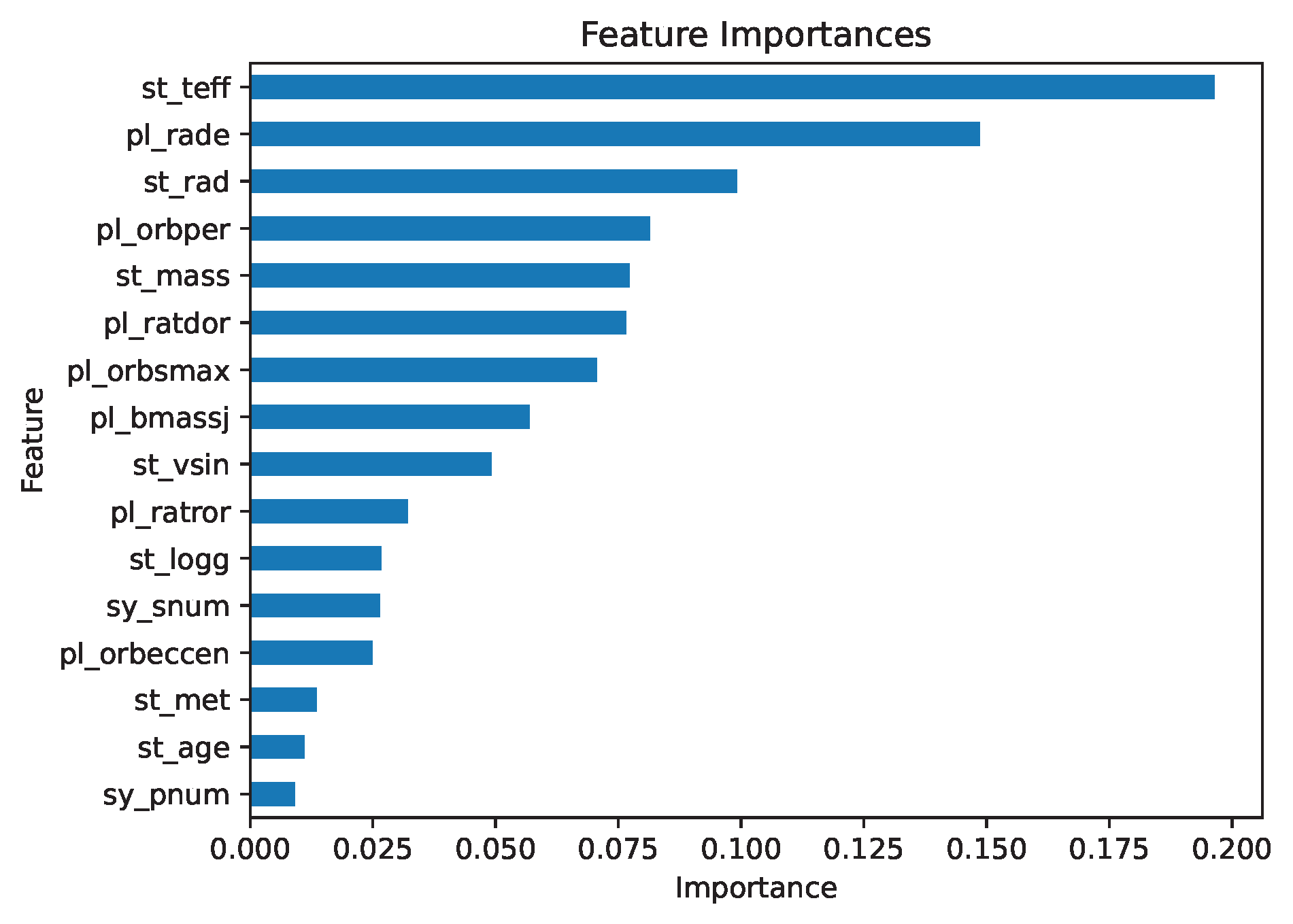
Despite the poor performance, examining feature importance can offer insights for improving the model. The feature importance plot highlights stellar effective temperature (st_teff) as the most influential feature, agreeing with Pearson and Spearman correlation metrics, which also identified effective temperature as strongly correlated with obliquity.

 

Predicted versus measured orbital obliquity from the random forest regression model. The predicted obliquities were produced using the testing dataset features and the measured obliquities are the actual obliquities from the testing dataset, with the original dataset split 70/30 between training and testing. The red dashed diagonal line is the one-to-one relationship between predicted and measured obliquities, points along the line indicate that the predicted obliquities agree with the true values while points off the line indicate a disagreement. Image credit: Brett Addison.

 

Feature importance plot showing the relative importance of each of the features used in training the random forest regression model. The stellar effective temperature (st_teff) appears to be the most important feature in the model. Image credit: Brett Addison.

 

More Robust Evaluation of Model Performance Using K-fold Cross-Validation

Previously, I evaluated the model using a simple train-test split. However, this approach is not ideal for small datasets, as performance can vary significantly depending on the split. To address this, I used k-fold cross-validation, a more statistically robust method. In k-fold cross-validation, the dataset is divided into k segments (folds). The model is trained and evaluated k times, with each fold serving as the test set once while the remaining folds are used for training, providing a comprehensive evaluation of the model performance. For example, in 10-fold cross-validation, the dataset is split into 10 folds and then evaluated 10 times using a different fold as the testing set for each iteration. A visualization of k-fold cross-validation is shown below.

 

Illustration of k-fold cross-validation, where the dataset is split into k-folds (or groups). There are k iterations and at each iteration, a different group is used as the testing set while all the other groups are used for model training. Image credit: Gufosowa, Wiki Commons.

 

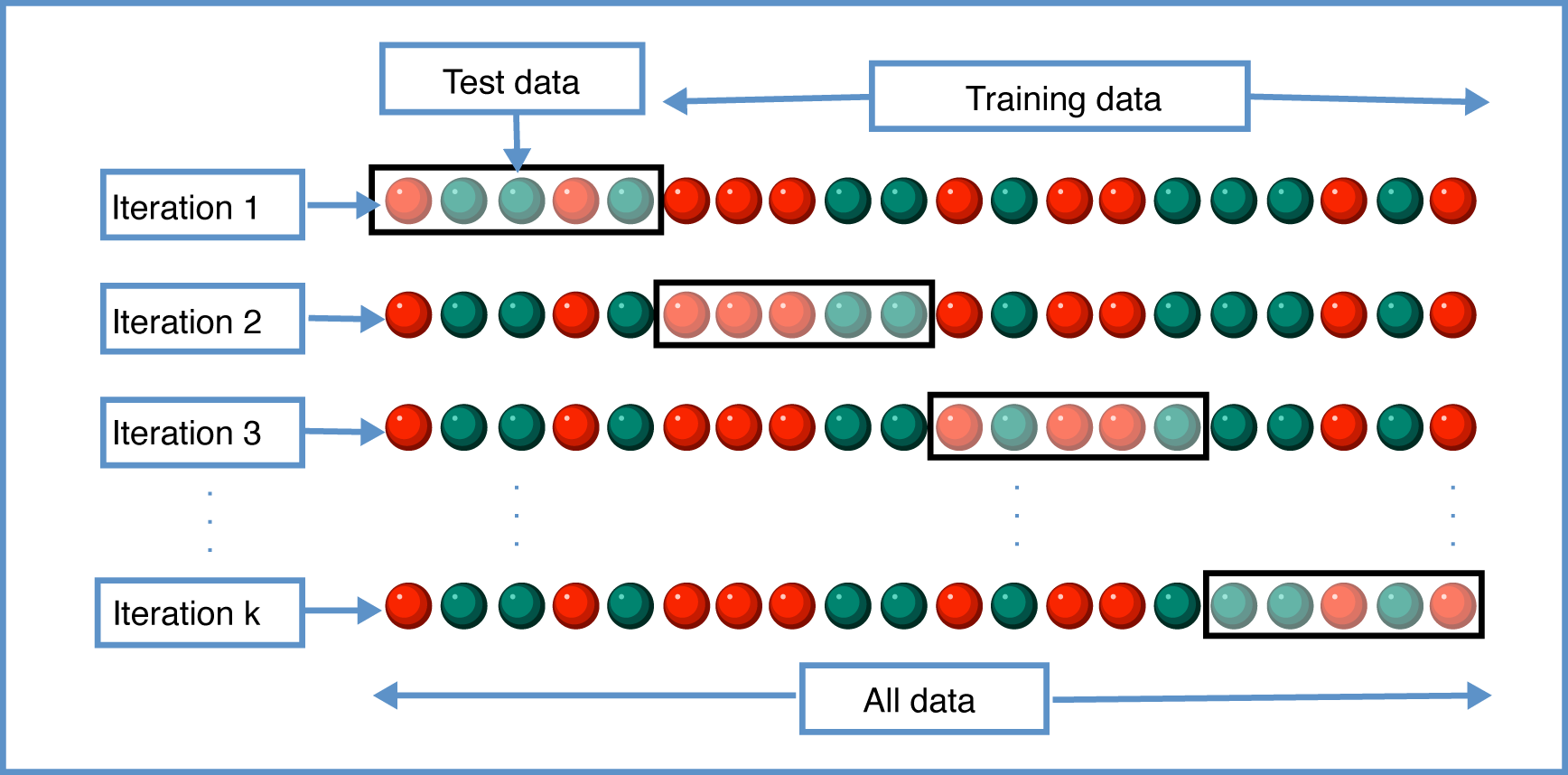
I performed 10-fold cross-validation, a commonly recommended choice that balances computational efficiency and model performance evaluation as well as provide a good balance between high variance (when having only a few folds) and high bias (having many folds, e.g., see detailed discussion on datacamp). To avoid data leakage, the dataset was split into folds before augmentation using a custom function, custom_cross_validation, which incorporates Scikit-learn's KFold function.

 

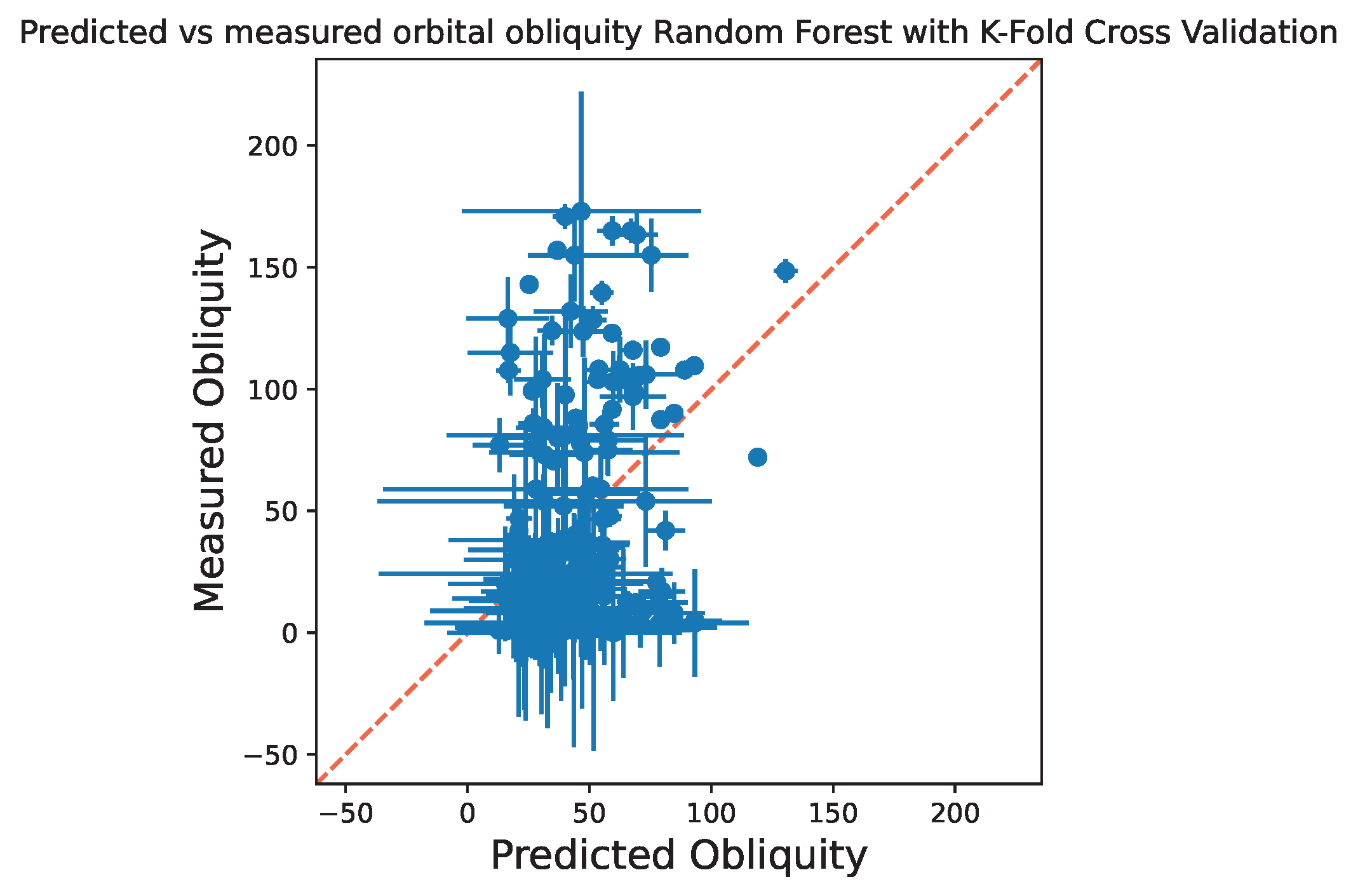
After splitting and augmenting the dataset, I trained and tested the random forest regression model on the 10 cross-validation iterations, calculating the same metrics as in the simple train-test split. To evaluate overall performance, I calculated the minimum, maximum, median, mean, and variance of the R² scores across the 10 fold iterations. Results showed a high variance of 0.52, with a minimum R² of -1.68 (worst performing model), a maximum of 0.64 (best performing model), a mean of -0.11, and a median of 0.22. This suggest the model’s performance depends heavily on the specific data sample used for training and testing.

 

Two likely reasons for this variability are: (1) the dataset is imbalanced, with about two-thirds of planets on low-obliquity orbits, and (2) the features used are weak predictors of obliquity. Both factors likely contribute to the model's limited performance. Below, I have plotted predicted vs. measured obliquities across all 10 folds, showing that most points do not align with the diagonal, further illustrating the model's challenges in accurately predicting obliquity.

 

Predicted versus measured orbital obliquity from the 10-fold cross validation random forest regression models. The predicted obliquities were produced from each of the dataset folds. The red dashed diagonal line is the one-to-one relationship between predicted and measured obliquities, points along the line indicate that the predicted obliquities agree with the true values while points off the line indicate a disagreement. Image credit: Brett Addison.

 

Although the model’s predictive power was limited, the project provided several valuable insights:

• The importance of robust and comprehensive datasets: The model’s performance highlights the need for a larger, more complete dataset with smaller uncertainties. This challenge is common in astronomy, where data can be sparse and have large uncertainties, and is equally critical in data science applications.
• Addressing dataset imbalances: Imbalanced datasets can bias machine learning models, making it difficult to achieve accurate predictions across a broad range of outcomes. Ensuring balanced representation within the dataset is crucial for reliable model performance.
• Feature selection and relevance: Including features that strongly correlate with the target variable—in this case, orbital obliquity—is fundamental for building an accurate and robust model. Irrelevant or weakly related features can dilute the predictive power of the model.
• Deep understanding of data: A thorough understanding of the dataset, including the physical relationships and correlations among features, is essential before applying machine learning techniques. This step ensures that the model is grounded in the physics and context of the problem, rather than purely statistical patterns.

 

Summary and Next Steps

This project demonstrates the potential and pitfalls of applying machine learning techniques to problems in astronomy and data science. While data-driven approaches offer the potential to uncover new insights, their success depends heavily on integration with domain-specific knowledge (thorough understanding of the data and the problem), especially when working with sparse or noisy datasets. Future efforts could focus on expanding the sample of data (in particular when new data sources become available), optimizing feature selection and/or engineering new features to better capture relevant patterns, or implementing other advanced machine learning models better suited to this problem to enhance predictive accuracy.

 

In the upcoming Part 3 of this blog series, I will share the steps I’ve taken to refine the random forest regression model and improve its performance—stay tuned!

 

 

Summary of the skills applied in this work: Python programming, Table Access Protocol (TAP), Application Programming Interface (API), Structured Query Language (SQL), Data Exploration, Data Visualization, Handling Missing Values (Data Imputation), Data Augmentation, Machine Learning, Random Forest Regression, K-Fold Cross-Validation.

 

 

 

< Previous Post   |   Data Science Home Page ⌂   |   Next Post (coming soon) >