Predicting the Orbital Obliquities of Exoplanets Using Machine Learning
What are Exoplanets?
Extrasolar planets (exoplanets) are planets that orbit stars outside of the Solar System. I have been truly fascinated by the sheer diversity of exoplanets that have been discovered in my field of research over the past three decades. Nearly all of the over 5,000 exoplanets discovered to date look nothing like the planets we have in the Solar System (check out the NASA Exoplanet Archive for the latest tally)! These planets range from scorching "hot Jupiters"--Jupiter-sized planets that whip around their star in only a few days--to super-Earths and mini-Neptunes (planets between the size of Earth and Neptune), and even planets that orbit around their parent star backwards (retrograde). This incredible variety contrasts starkly with the orderly configuration of the Solar System, where planets follow near-coplanar orbits aligned with the Sun's equator.
This raises an intriguing question: Is the Solar System unique?
How Are Exoplanets Detected?
To address this question, I will first cover the two primary methods of discovering exoplanets and their detection biases. These two methods are the transit method and the radial velocity method (see the excellent review of exoplanet detection methods by Jason Wright and Scott Gaudi).
- Transit Method: Astronomers monitor the brightness of stars for any periodic dips caused by planets passing in front of their stars. This technique has been the most successful in finding planets to date (thanks to space-based missions such as Kepler and TESS), though it is biased towards detecting larger planets that orbit closer to their host star (higher probability of transits and larger dips in brightness make them easier to detect).
- Radial Velocity Method: By observing the back-and-forth motion (periodic Doppler shift) of a star's light, caused by the gravitational "wobble" of an orbiting planet, astronomers can infer the presence of a planet. You can think of Doppler shift with the example of a police siren, the pitch of the sound increases (shorter wavelengths) when the police vehicle is approaching while the pitch decreases (longer wavelengths) when the vehicle moves away. Similarly, the gravitational effect of an orbiting planet will cause its star to move towards and away from the observer (as the star orbits around the center-of-mass of the system), causing the star's light to be blue-shifted (shorter wavelengths) and red-shifted (longer wavelengths), respectively. This method was used to discovery the first exoplanet orbiting a Sun-like star (51 Pegasi b, see, Mayor & Queloz 1995) and has since been used to detect nearly a 1000 exoplanets. The radial velocity technique, however, is biased towards detecting massive planets on short-period orbits, as such planets produced larger wobbles over shorter periods of time, making them easier to detect.
These detection biases partly explain why most discovered exoplanets differ so drastically from those in the Solar System. However, recent studies suggest that the Solar System may indeed be somewhat unique (e.g., see Mishra et al. 2023a and Mishra et al. 2023b).
Orbital Obliquity: A Window into Planetary Formation & Migration
One intriguing clue regarding the Solar System uniqueness lies in the orbital obliquities of exoplanet, the angle between a planet's orbital plane and its host star's equator. This measure, also known as spin-orbit alignment (e.g., see, Rossiter 1924, McLaughlin 1924, Queloz et al. 2000, and Addison et al. 2013), offers insights into planetary formation and migration histories (see the review by Dawson & Johnson 2018) and is a topic I have studied quite extensively as an astronomer (see my papers on this topic, e.g., Addison et al. 2018 and Addison et al. 2021).
Before the discovery of the first exoplanets, it was predicted that Jupiter mass planets would be found on long period orbits while rocky terrestrial type planets would be found much closer in, as observed in the Solar System. This assumption was based on the core-accretion model of planet formation that was developed, in part, based on the morphology of the Solar System. It was quite a surprise to most astronomers when the first exoplanets discovered were hot Jupiters.
The core-accretion model does not predict the existence of hot Jupiters, but instead predicts Jupiter mass planets forming beyond the so called 'ice-line' (about the distance of Jupiter to the Sun in the Solar System). This is where icy materials can exist in a solid state and clump together to build giant planets. To explain the existance of hot Jupiters, it is thought that these planets initially formed out beyond the ice-line and then migrated inwards, with their migration shaping their spin-orbit alignment.
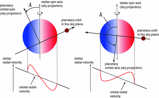
A planet's orbit is considered aligned if the measured angle between its orbit and its host star's equator is consistent with zero degrees. The diagram below illustrates orbital obliquity for two scenarios, a planet on a somewhat misaligned orbit and a planet on a retrograde orbit. It should be noted that typically the 'sky-projected' obliquity (given as λ) is measured, not the true obliquity in 3D space (given as ψ). This is due to not knowing the orientation of the stellar spin axis.
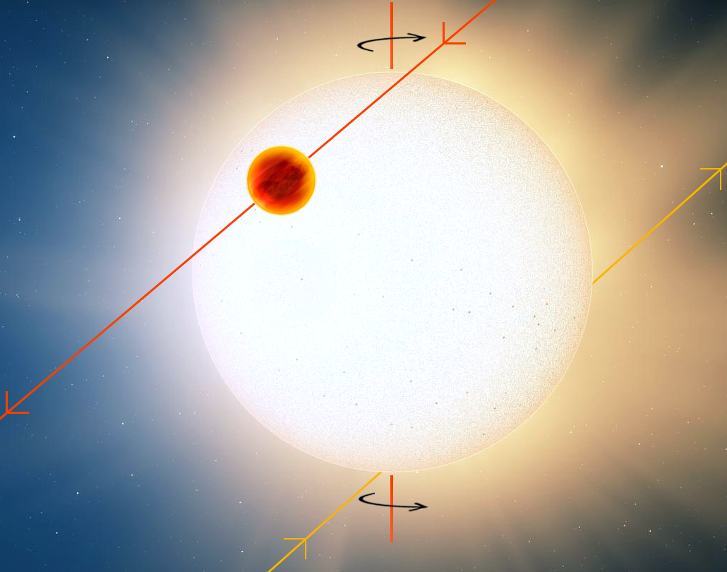
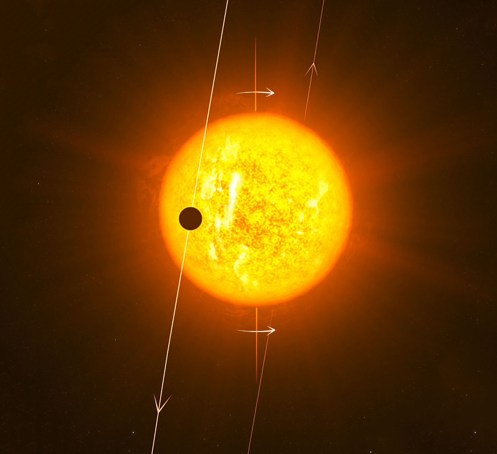
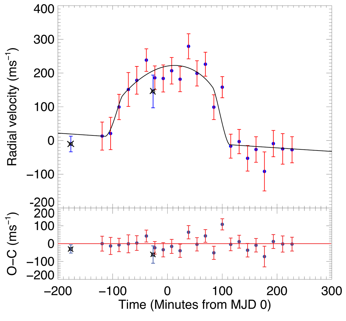
Obliquity has traditionally been measured through spectroscopy of transiting exoplanets, such as by measuring the radial velocity anomaly (the Rossiter-McLaughlin Effect, see below) or the distortion of the stellar line profile produced during a transit (Doppler tomography). Below on the left is an artist impression of the hot Jupiter, WASP-79b, with its orbit misaligned by close to 90° (near polar orbit) and on the right, the Rossiter-McLaughlin Effect velocity anomaly as measured for WASP-79b, given in Addison et al. (2013). A video animation, also shown below, illustrates how the radial velocity anomaly is produced when a planet transits its star.
The sample of planet's with measured obliquities has grown in recent years with nearly 230 planets listed in the TEPCat catalog. This is sufficient to allow us to explore potential correlations between planetary and stellar properties and orbital obliquity. For instance, there is evidence for a positive correlation between a star's temperature and a planet's orbital obliquity (first noted by Winn et al. 2010 and extensively studied by others, e.g., see review by Albrecht et al. 2022).
Using Machine Learning to Predict the Orbital Obliquities of Exoplanets
Machine learning offers a powerful tool to uncover patterns in complex datasets. In this blog post series, I'll outline how I've used machine learning, specifically random forest regression and classification, to predict exoplanet orbital obliquities based on their physical properties.
Data Science Home Page ⌂ | Next Post >