Predicting the Orbital Obliquities of Exoplanets Using Machine Learning

Illustration of a decision tree (in this case the first tree in the forest) with a depth of three branches from the random forest classifier model produced using the training dataset. A high-resolution pdf is available to download by clicking on the image. Image credit: Brett Addison.

 

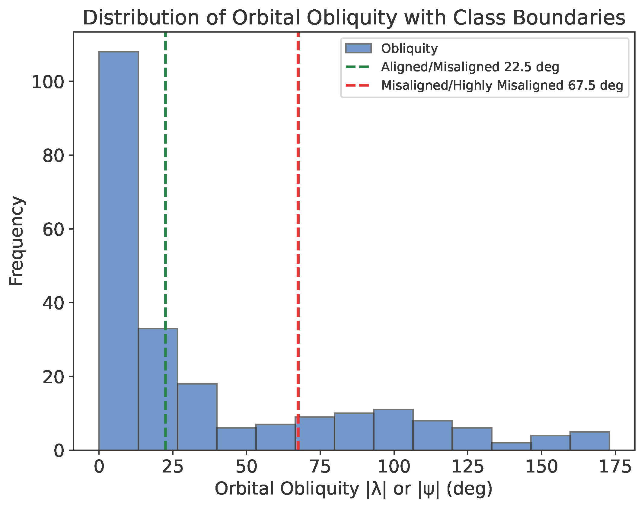
In my previous posts (Parts 2 and 3), I discussed using a random forest regression model to predict exoplanet orbital obliquities based on stellar and planetary parameters. However, its predictive accuracy was limited. In this post, I shift to a classification approach using Scikit-learn's RandomForestClassifier, categorizing obliquities into aligned (λ < 22.5°), misaligned (22.5° ≤ λ < 67.5°), and highly misaligned (λ ≥ 67.5°)—following how they are defined in Addison et al. (2013).

 

Data Preparation and Feature Engineering

The dataset is compiled using the same preprocessing steps as before, including replacing missing values using physically derived estimates instead of median imputation as well as using the same engineered features—planet-to-star mass ratio (pl_ratmom) and planet density (pl_density), as discussed in Part 3). To account for uncertainties, I again augment the dataset by simulating 100 additional data points per row based on the 1 σ errors.

 

Before training the random forest classifier model, it’s a good idea to get a sense of the distribution of orbital obliquities across the three categories, as defined above. The plot below shows the distribution of obliquities, revealing a class imbalance: ~60% of planets are aligned, while only ~15% fall in the misaligned category. This imbalance could impact model performance by introducing bias into the model predictions, a challenge I address later.

 

Distribution of orbital obliquity with classification boundaries. λ < 22.5° are aligned (left of the green dashed line), 22.5° ≤ λ < 67.5° are misaligned (between the green and red dashed lines), and λ ≥ 67.5° are highly misaligned (right of the red dashed line). Image credit: Brett Addison.

 

Model Training and Evaluation

The dataset is split 70/30 for training and testing, with augmentation applied only to the training set to prevent data leakage (as discussed in Part 2). The model is then trained using the training set and evaluated on the testing set using the standard classification metrics accuracy, precision, recall, and F1-score, averaged across the three classification categories. The metrics were calculated using the Scikit-learn functions accuracy_score, precision_score, recall_score, and f1_score. The model performance results are:

 

 

What Do These Metrics Mean?

• Accuracy: The proportion of total predictions that are correct.
• Precision: Of all predicted positive cases, how many are actually positive? High precision means fewer false positives.
• Recall (Sensitivity): Of all actual positive cases, how many were correctly predicted? High recall means fewer false negatives.
• F1-score: The harmonic mean of precision and recall, balancing both metrics.

 

While these scores appear promising (≥0.8 is generally considered good, see discussion by Stephen Walker II), a closer inspection of the class-wise performance paints a different picture, in particular for the misaligned and highly misaligned categories:

 

 

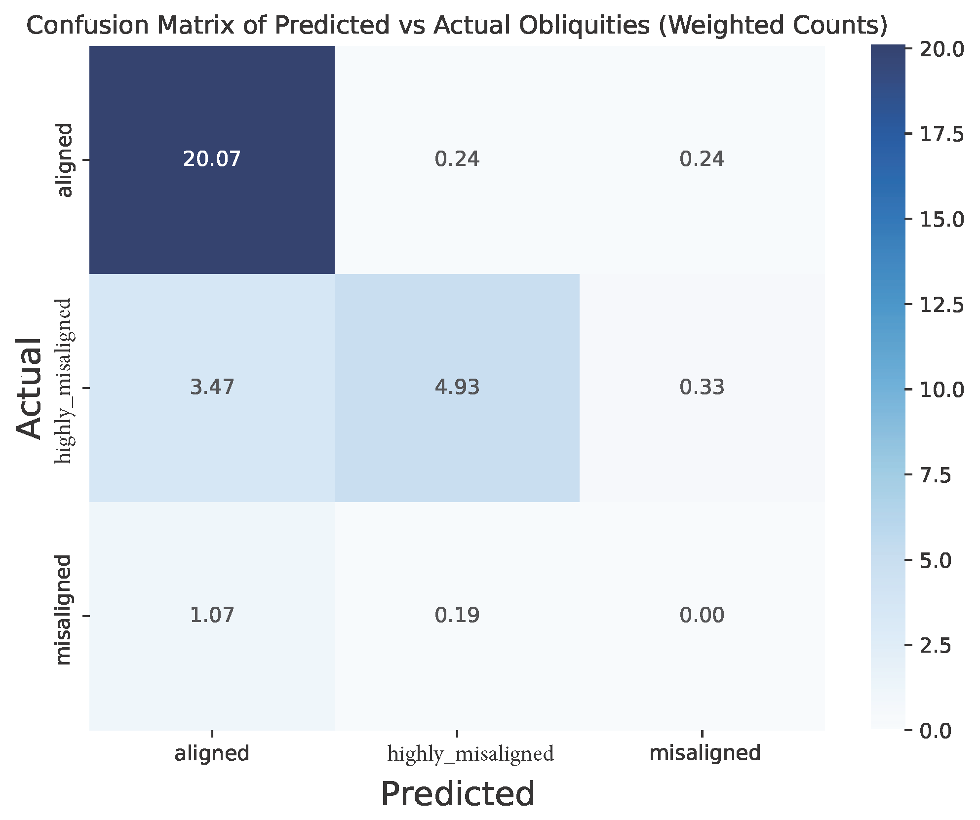
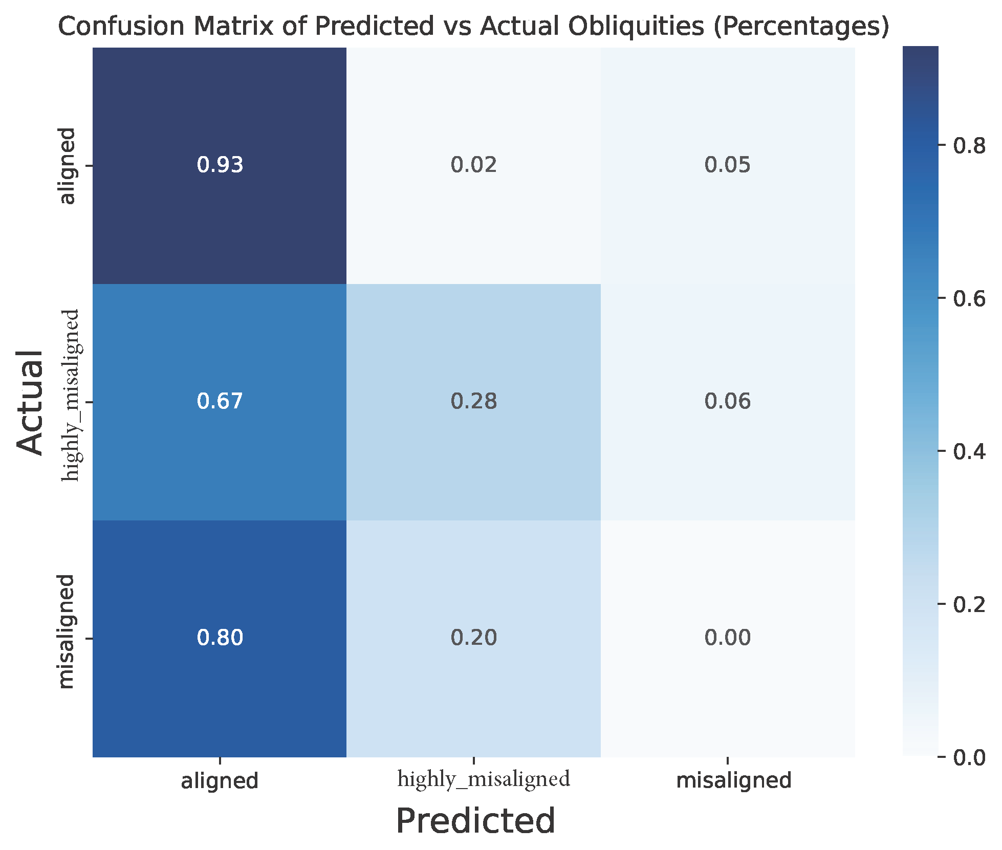
The table above indicates that the classifier fails entirely to predict misaligned planets, with metric scores of 0. This is also visually reflected in the confusion matrices below, which shows how well the classification model has performed. For reference, the rows of the matrix represent the actual values, the columns are the predicted values, and the diagonal are the correct predictions. The values outside the diagonal indicate the occurance of wrong predictions.

 

Confusion matrix of the weighted counts from the random forest classifier model of the predicted versus actual orbital obliquities. The counts along the diagonal (top left to bottom right) are the weighted number of correctly predicted classifications while all other cells are the weighted number of incorrect classifications. Image credit: Brett Addison.

 

Confusion matrix similar to above but in terms of percentages from the raw counts (unweighted counts not taking the obliquity uncertainties into account). Image credit: Brett Addison.

 

Insights from Feature Importance and Model Limitations

Examining feature importance, stellar effective temperature (st_teff) is the most significant predictor, but multiple features contribute nearly equally, suggesting a complex parameter dependency.

 

Feature importance plot showing the relative importance of each of the features used in training the random forest classifier model. The stellar effective temperature (st_teff) appears to be the most important feature in the model though several other features are almost equally important. Image credit: Brett Addison.

 

The poor performance in correctly classifying the orbital obliquities of planets is likely due to:

• Severe class imbalance: There are significantly more planets that are in the aligned class compared with the aligned class.
• Small overall sample size: Small sample size limits the model's ability to fully explore the parameter space.
• Weak feature-obliquity correlations: As seen in the regression models, there is a lack of strong correlations between the features and orbital obliquity.

 

To verify these results, I conducted 10-fold cross-validation, which showed slightly better (though still poor) performance across models, likely due to different training/testing splits in each fold.

 

Next Steps

Given the classifier's struggles with three categories, a binary classification approach (aligned vs. misaligned) might yield better results. In the next post (coming soon), I will explore this strategy, so stay tuned!

 

 

Summary of the skills applied in this work: Python programming, Data Visualization, Machine Learning, Random Forest Classification, K-Fold Cross-Validation.

 

 

 

< Previous Post   |   Data Science Home Page ⌂   |   Next Post (coming soon) >